Seismic Refraction Case Study:
This report discusses a seismic survey I did for the Stillwater
Mine at the Hertzler Ranch proposed tailings impoundment site.
The survey was designed to evaluate the valley sediments and attempt
to locate bedrock depths by measuring both P-waves (primary or
pressure waves) and S-waves (secondary or shear waves). P-waves
oscillate in the same direction of motion and S-waves oscillate
perpendicular to the direction of motion (SV
for vertical motion and SH for horizontal
motion). Poisson's ratio (sigma) is the ratio of transverse strain
to longitudinal strain and can be represented as sigma=(VP^2-2VS^2)/2(VP^2-VS^2). This shows accurate measurements of the
P-wave and S-wave velocities can be used to estimate the strength
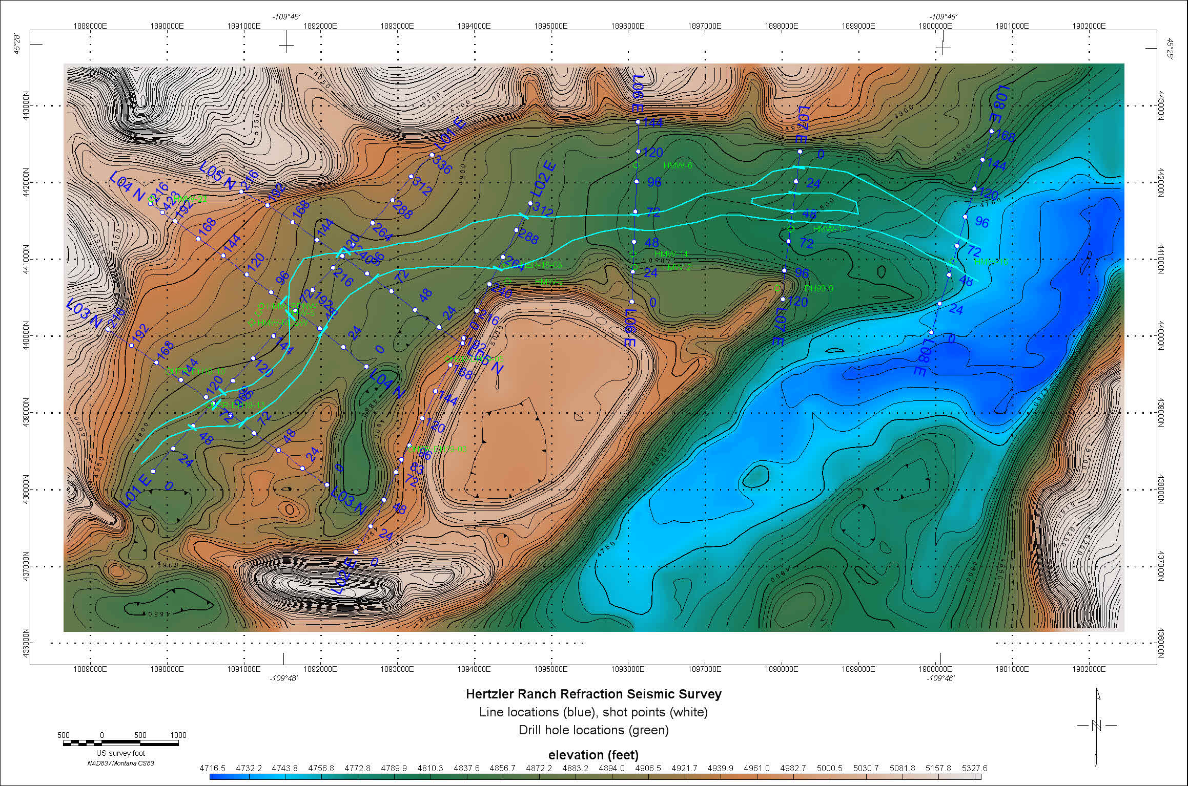
of the soil. The survey consisted of eight lines (Fig. 1) of various
lengths.
Figure 1: Line locations for the valley shown in blue. Shot point locations are indicated by white circles and drill holes with logs for comparison to the seismic sections are shown in green.
The receiver array consisted of 120 geophones separated by 5 meters. Shot points were taken at every 24th geophone. Data quality was generally good, but a different group was drilling for cone penetrometer measurements at the same time which introduced additional noise into the data. Most shots were taken using a 550 lb. weight drop mounted on a trailer. In more rugged terrain a 88 lb. weight drop was used, and finally at the ends of the lines in the hills a 16 lb. sledge hammer was used (Fig. 2).
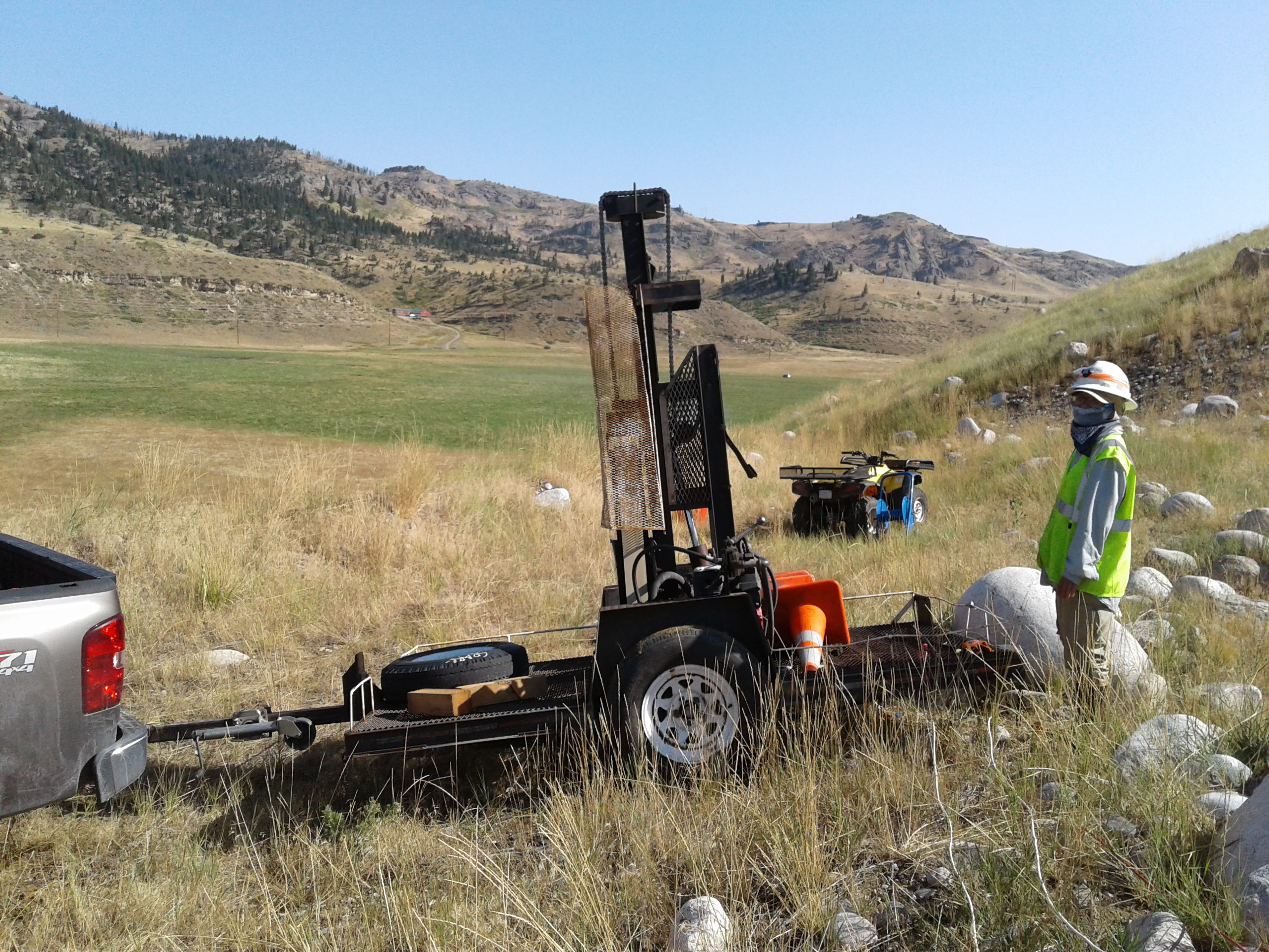
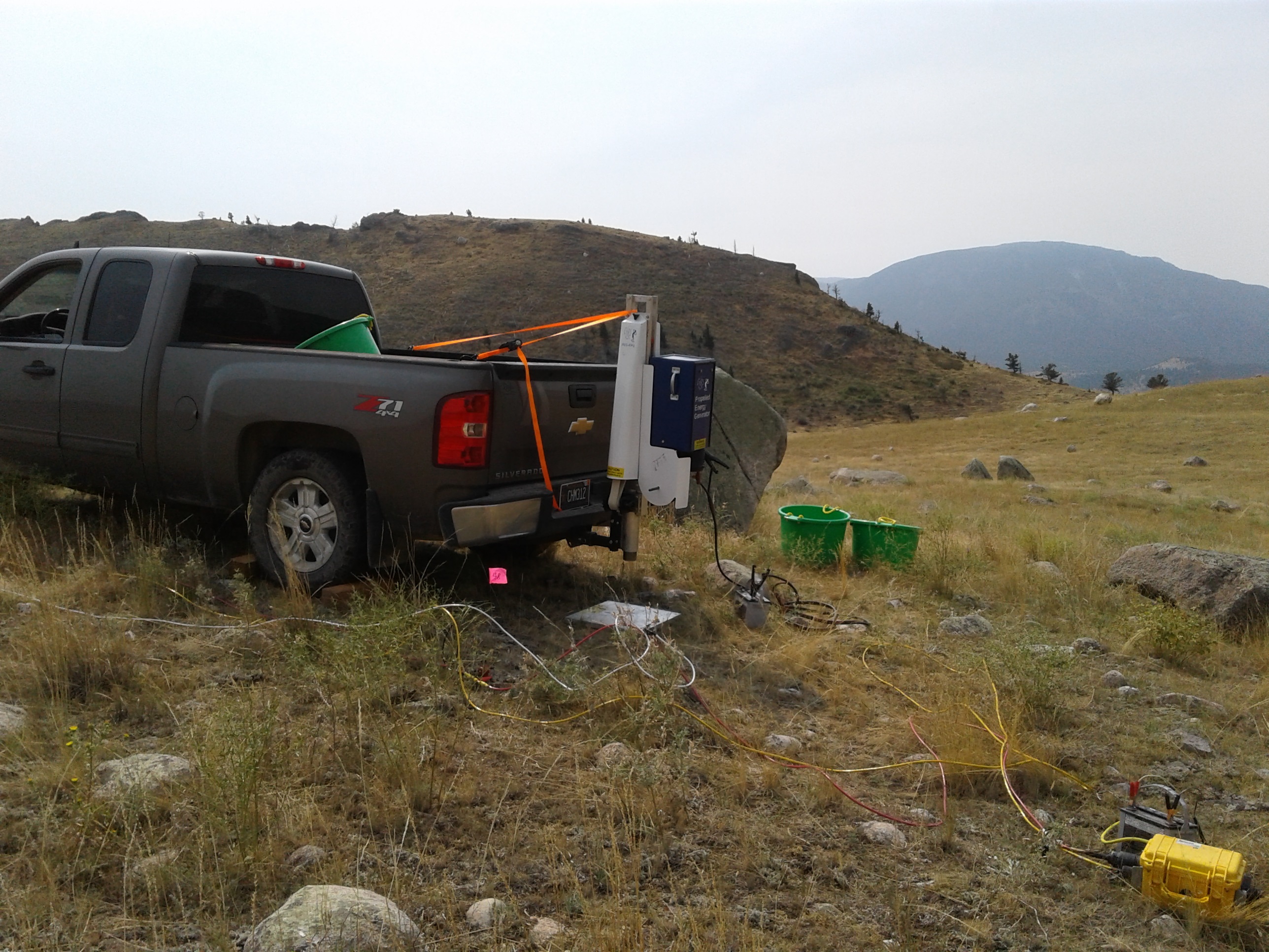
Figure 2: Trailer mounted 550 lb. weight drop and trailer hitch mounted 88 lb. weight drop. Both are accelerated by elastic bands. The yellow box in the second photo is one of the five seismographs used.
The seismic method provides a wealth of information and there are various processing techniques that utilize various segments of these data (Fig. 3). The primary purpose of this survey was to establish depth to bedrock. For refraction processing, you can achieve a depth of penetration approximately equal to 1/6 of the array length. Our array length (aperture) was 600 meters (1969 feet) so the depth penetration was approximately 100 meters (328 feet). I utilized a refraction processing technique for the P-wave data and a frequency transform technique for the S-wave data. The refraction program used is called Rayfract is written by Siegfried Rohdewald and is a modification of the standard ray tracing algorithms to incorporate diving tomographic rays. The frequency transform program used is a MASW (multichannel analysis of surface waves) program designed by the group at the Kansas Geological Survey. This program is better suited to defining the stratagraphic differences in the alluvial overburden. Since the MASW relies on the "ground roll" Rayleigh waves that propagate at the earth's surface, the depth penetration is limited to about 40 meters (130 feet) because the wave decays exponentially with depth.
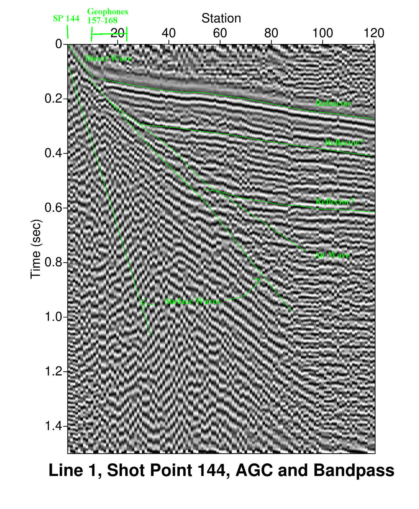
Figure 3: Shot point 144 on Line 1 which has had automatic gain control and bandpass filtering applied to emphasizes the response of reflectors and refractors. The seismic trace shows responses from the direct wave (P-wave that travels at the surface), rrefractor (P-wave) and possible aditional reflectors (P-wave). Also noted are the air wave (P-wave that travels through air, approxiate velocity of 340 m/sec or 1100 ft/sec) and the ground roll or surface wave (S-wave that travels at the surface). In general the S-wave velocity in any given rock is roughly 1/2 of the P-wave velocity.
Rayfract:
In all cases I used the wavefront refraction method to generate
an initial layer model based upon standard refraction surveying
techniques and then used WET (Wavepath Eikonal Traveltime) diving
wave frequency dependent tomography to add detail and depth penetration
to the initial model. This method seemed to best match the well
logs and produced more realistic sections when compared to the
surface geology.
Figure 4 shows the refraction time picks for Line 1 in blue. For refraction processing only the travel time to the first interfaces are used. No amplitude information is used. wave velocity.
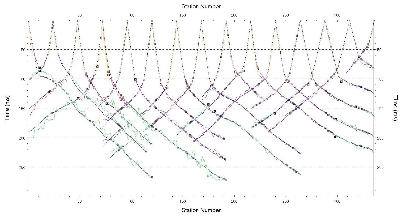
Figure 4: First break picks (in blue) for each of the shot points on Line 1. Squares mark picks for different layers. The inverted data are shown in orange (direct wave), red (first refractor), and green (second refractor).
Each break in slope represents a different velocity (marked by squares). If the earth was made of homogeneous layers, the blue lines would be straight between the squares. The data were first modeled with two layers using the wavefront method. This produces a two layer model (fig. 5) for the Rayfract tomographic inversion. The difference between the orange, red, and green lines compared to the blue lines show the error in the fit. The final tomogram produced by Rayfract is shown in Figure 6. The Rayfract tomograms are primarily P-wave models since they are based upon refraction processing. However when they use some lower frequencies in the tomographic inversion, they are including some S-wave energy so the P-wave model velocities may be slightly lower than the true P-wave response particularly at depth. The velocities at depth from this method may appear slightly lower than those measured by a cone penetrometer. It looks like the first refractor may represent the water table and the second refractor is the bedrock.
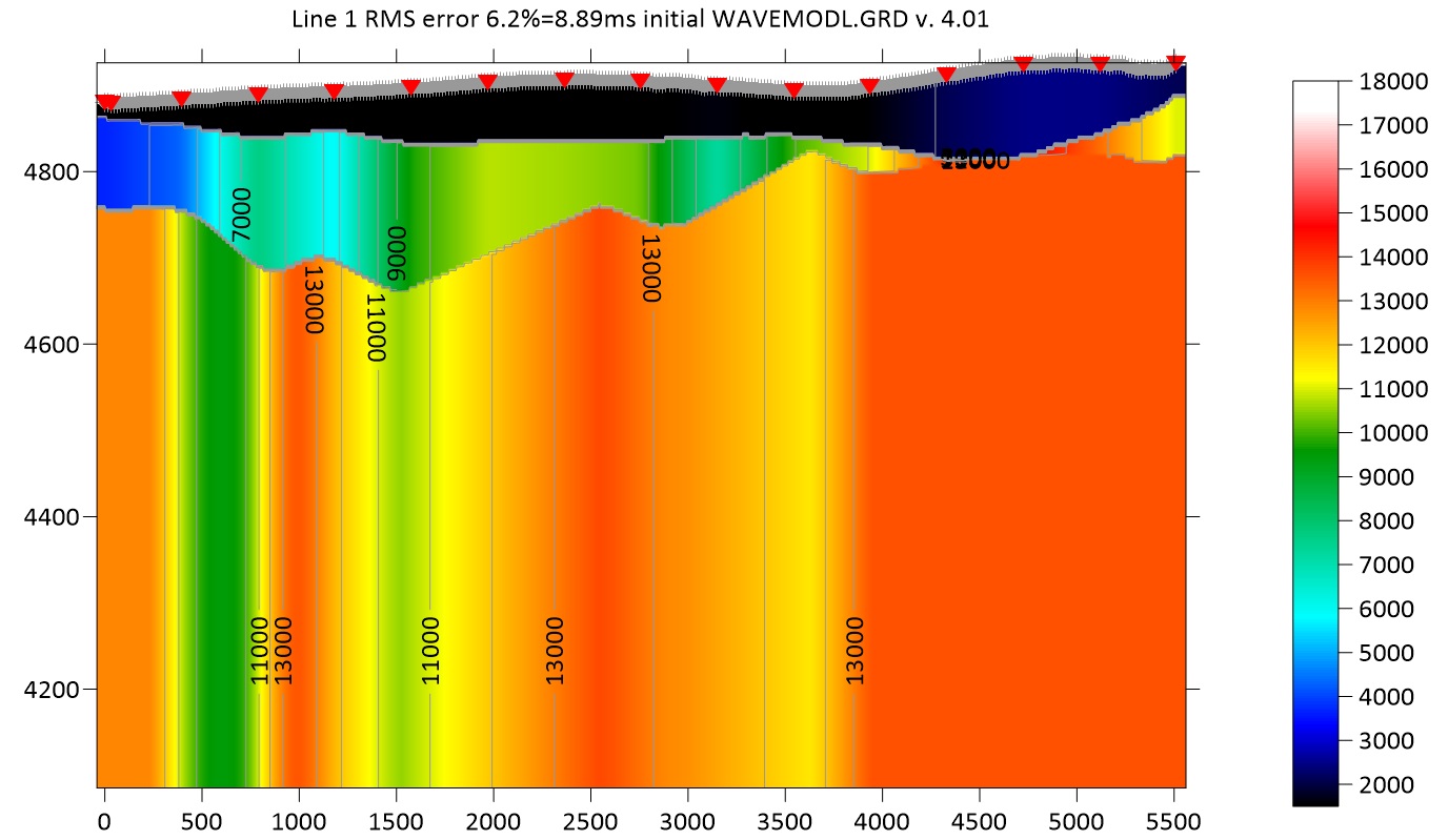
Figure 5: Initial model created after the wavefront refraction interpretation of two refractor interfaces. This model is used as input for the WET inversion produced by the Rayfract software. Shotpoints are shown by red triangles and geophone locations by gray circles.
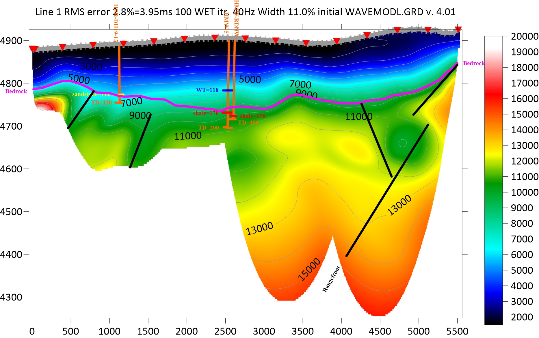
Figure 6: Line 1 P-wave inversion with interpreted faults (black), bedrock (magenta), and drillholes (orange). Lithology in the dirllholes for sandstone bedrock (yellow), shale bedrock (red), and water table (blue). All distances and elevations are in feet and all velocities are feet/sec.
MASW:
The MASW method uses the surface ground roll to solve for the
S-wave velocities in the near surface. Most of the ground roll
response is a special SV wave called the
Rayleigh wave. This wave travels at approximately 92% the speed
of other S-waves so velocity estimates from this technique may
be slightly lower than measured by a cone penetrometer. The geophones
used should be a distance of approximate 40 meters from the source
so the source appears as a plane wave. Then care should be taken
to select the data that are just part of the surface wave response
(fig. 7). These time-distance data are then transformed to frequency-velocity
domain via either a Fourier or a Radon transform. The surface
wave and the reflection and refraction energy plot at different
locations in the frequency-velocity space. Once transformed to
the frequency space, the surface wave energy responses are picked
by the user (fig. 8). These responses are then inverted by the
software for a one dimensional inversion (fig. 9). Once all of
the 1D inversions are completed, the results are stitched together
into a 2D profile of the S-wave velocity (fig. 10).
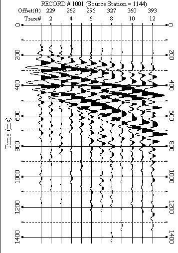
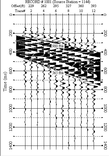
Figure 7: Geophone records 157-168 for shot point 144 without gain or bandpass filtering. The MASW software automatically selects the largest amplitude traces for transforming to frequency-velocity domain. Since the largest response is caused by the surface wave, most of the energy transormed is the Rayleigh wave data.
(1001).JPG)
Figure 8: Radon frequency-velocity transform of the data from fig. 7. The picks for the fundamental mode and the first two harmonic modes are shown by black lines. The responses below the fundamental mode are noise caused by spatial aliasing.
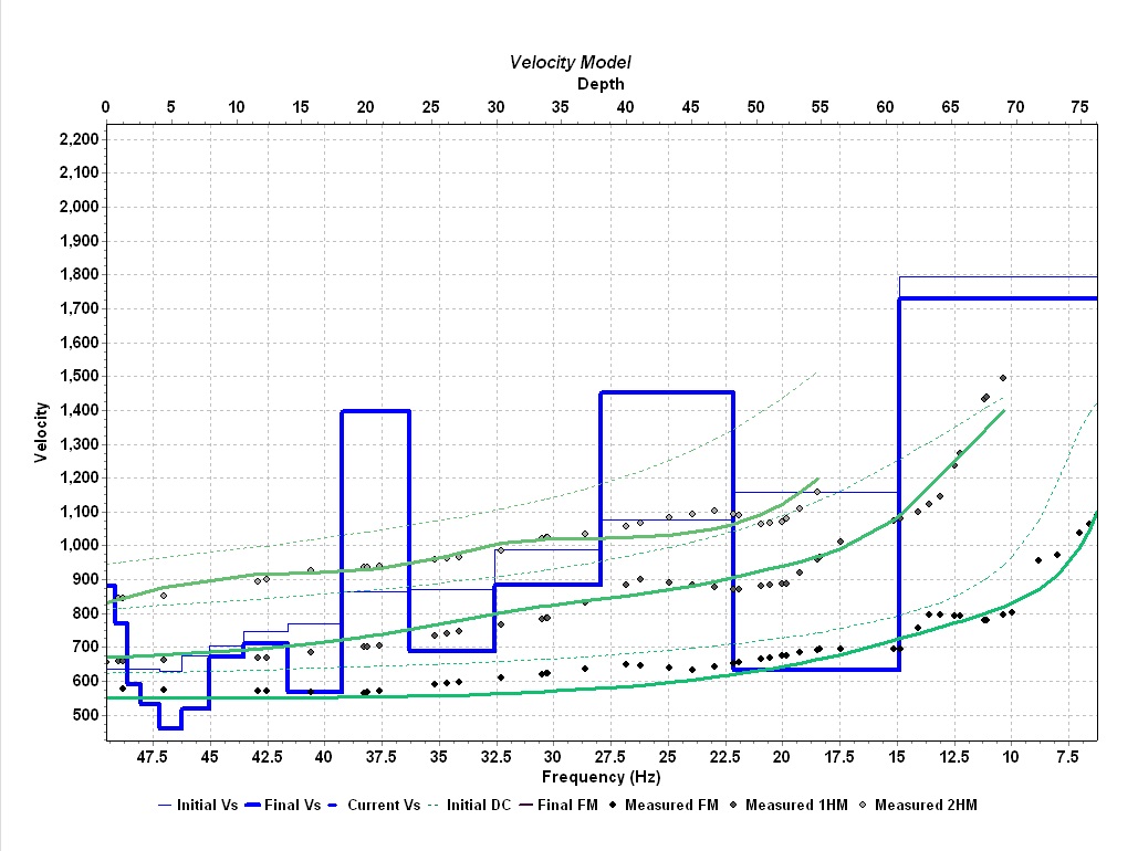
Figure 9: 1D inversion using 15 layers of the three modes picked from fig. 7 (black and gray dots). The initial frequency-velocity fit (dashed green lines), final frequency-velocity fit (solid green llines), initial velocity-depth model (thin blue line), and final velocity-depth model (thick blue line) are shown.
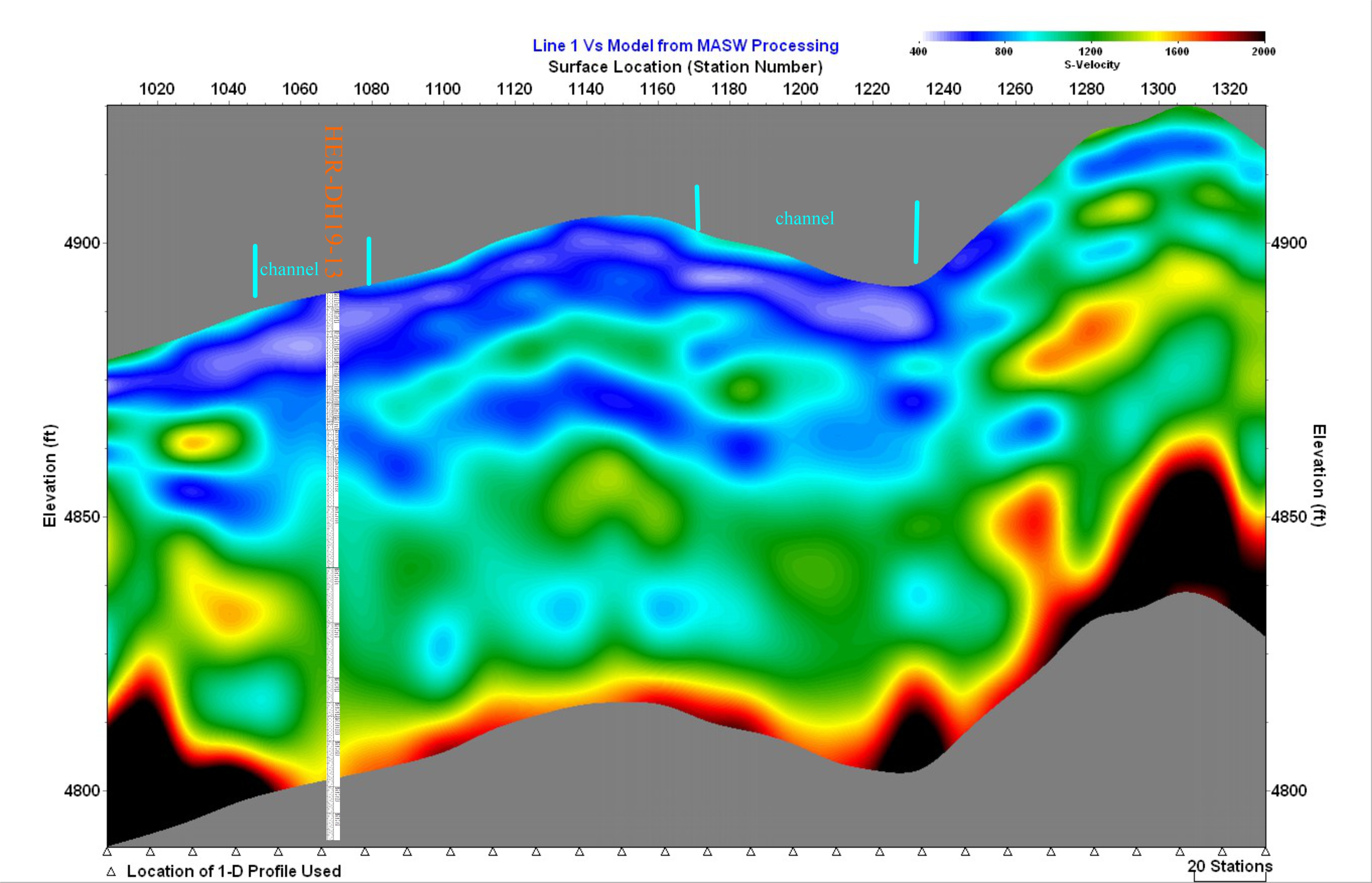
Figure 10: S-wave inversion for Line 1. The log for DH19-13 has been superimposed upon the section. Good stratagraphic layering is indicated in the image. Two possible paleochannels are marked based upon lower velocity values in the near surface data. All elevations and distances are in feet and all velocities are feet/sec.
Ideally a receiver spacing of 2 meters or less should be used for the MASW method. Some spatial aliasing does occur for larger receiver spacings. The surface wave produces one fundamental mode and multiple harmonic modes. For all soundings, I picked the fundamental mode and the first two harmonic modes. The harmonic modes help to better define near surface layers. I did not attempt to pick higher modes because if spatial aliasing occurs, it can produce spurious results that mimic higher harmonic modes. I compared the results using both the Fourier and Radon transforms. The Radon transform yielded sharper areas that made picking the S-wave response easier so I used it on all lines. As an example, the inversion of Line 1 consisted of 28 1D soundings.
The P-wave inversions for each of the lines show the error of the data fit (usually about 3%) after 100 iterations of the WET tomography based upon the initial wave model refraction processing. Line 8 had the largest error term and this may be caused by 3D effects from the river valley. The P-wave inversions really don't show much differentiation in the sedimentary section. They just show increased velocity with soil compaction at depth. Therefore I only picked depth to bedrock and some structural controls based upon these sections. The velocity for the depth to bedrock seems to be about 8500 feet/sec. on average, but near the surface it is much lower based upon drill intercepts. This is probably caused by weathering of bedrock when it is closer to the surface. Finally for quality control, I merged all of the datasets together so they could be plotted as fence diagrams (fig. 11). All of the cross sections are displayed with the same color scale. In general the velocities picked from one line agree well with the lines they intersect. I have enhanced this color scale to indicate the lowest velocity zones (gray/white colors). There are no significant low velocity zones on lines 2, 4, and 7.
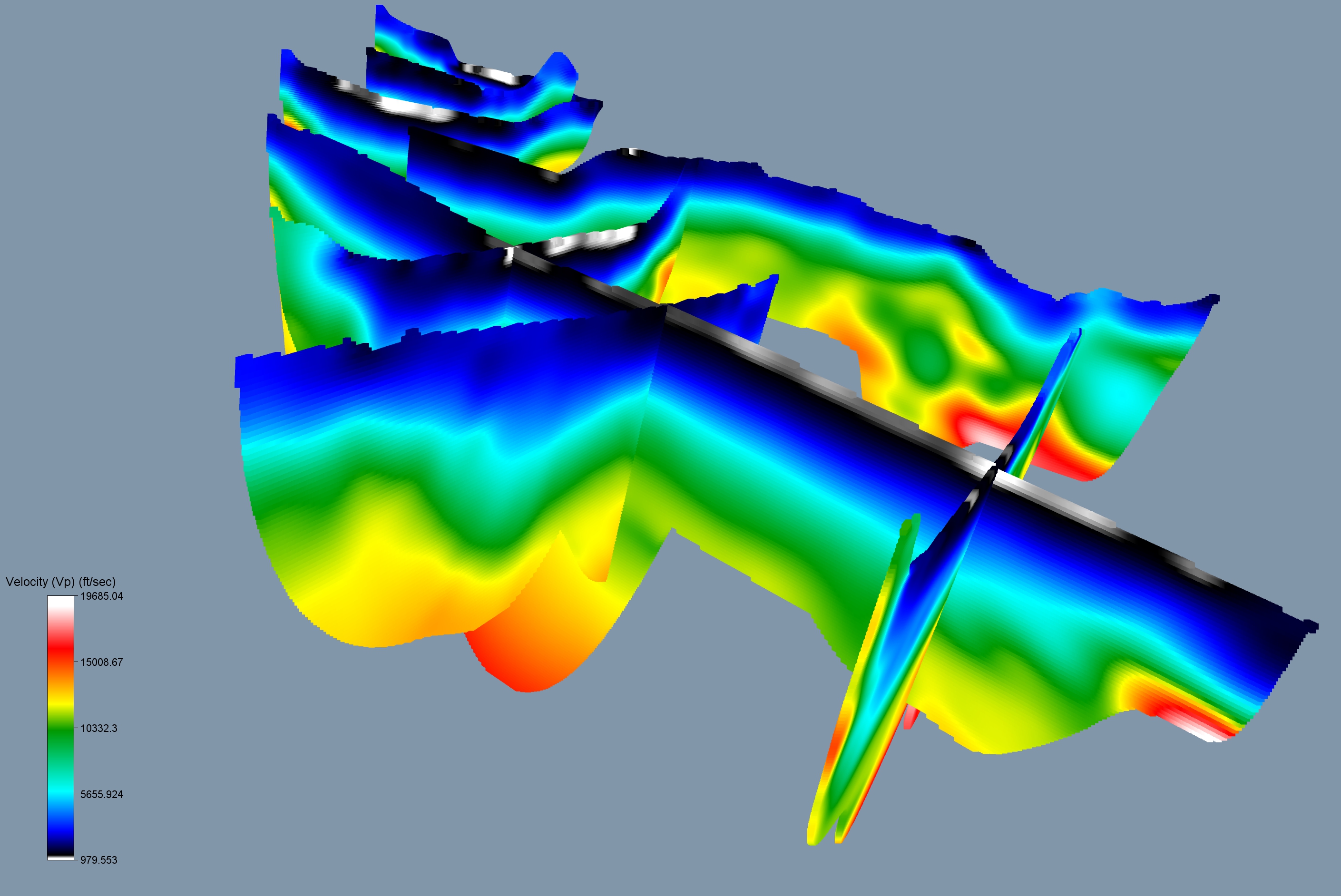
Figure 11: P-wave inversions viewed from the west. Lines 3, 4, and 5 are coming towards the viewer, Lines 1 and 2 are perpendicular to the viewer, and Lines 6, 7, and 8 are in the backgroThe S-wave inversions were created by stitching together multiple 1D inversions. For each 1D inversion 12 geophone records were used and the center of each group is indicated by the triangles at the bottom of each profile. Where the sections extend deep enough, there is generally good agreement with bedrock and increased velocities.
The S-wave inversions are much better suited from examining the sedimentary section than the P-wave inversions. I have compared the results with the drill logs and the low velocity zones agree pretty well with gravel and sand units while the higher velocity zones correspond with silts and clays. Of course with depth and soil compaction, all of the velocities increase. Line 1 shows the concerning image a near surface low velocity zone which is hidden under a thin high velocity layer. Line 1 shows good stratagraphic layering which should be expected for a profile that goes down the middle of the valley. All of the lines show some degree of layering with the exception of Line 2. I picked a possible paleochannel by mapping and connecting the near surface low VS zones (fig. 1). For quality control, I merged all of the datasets so they could be plotted in fence diagram format (fig. 12). All of the cross sections are displayed with the same color scale and the velocities agree very well where the lines intersect. This gives me more confidence in using these data to interpret the stratagraphic section. Note lines 5 and 6 have strong low velocity zones at the surface. These zones are slightly offset from the low VP zones on the same lines.
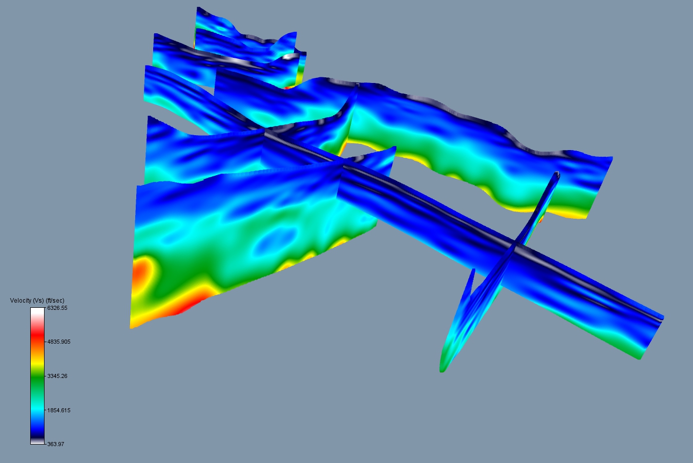
Figure 12: S-wave inversions viewed from the west using the same perspective as figure 11. Vertical exaggeration is 4x. Color scale has been enhanced to identify the lowest velocity zone (in gray/white). This zone is interpreted to be a possible paleochannel.
The P-wave inversions worked pretty well mapping the depth to basement based upon the well log data. However, in some steep areas, the inversion didn't adequately represent the sharp increase in bedrock elevation. The Rayfract program is more effective if you use a shot point at every third geophone. I should have used more shot points. There was also some variation because is some places the bedrock was shale and in others it was sandstone, which have different velocities. The S-wave inversion showed a consistent low velocity zone in the near surface that is interpreted to be a paleochannel. This allows the engineers to design stronger footings in these areas so the tailings impoundment will be stronger.
Results are presented with permission from Stillwater Mining.